Open311 Pipeline

Overview

A streaming pipeline that treats a language model’s judgement as a column in a warehouse. Chicago’s Open311 API is polled into Kafka. A consumer asks Claude Haiku 4.5 to give each service request an urgency tier — Critical, High, Medium or Low — with a confidence score and a one-sentence reason. The result is merged into DuckDB or Snowflake on the request ID, and dbt turns the rows into SLA compliance by category and month.

A second, batch path loads a full fiscal year from the city’s data portal: 2,124,780 requests created in federal FY2026, each day of the year verified against the portal’s own count. Measured over every request created that year, compliance is 44.8%. Measured the way the first version did it, over requests that had already closed, it is 51.0%.

The whole thing runs from a fresh clone with no accounts. make demo-local replays 300 real requests, with the labels Claude gave them, through Kafka, the consumer, the warehouse and dbt, then builds the fiscal-year marts from a committed sample of the portal data.

The problem

I built this to explore a question that matters more than which model to call: what does it take to put a model’s output inside a system people already rely on? A 311 feed is a good place to find out. It is an existing operational system, it publishes every request, and it already carries a form of accountability — requests get closed, and the time to close can be measured.

Urgency is not in the feed. When a model supplies it, urgency stops being an annotation and becomes an input to a metric: whether a request closed inside the window its tier allows. Once a model’s label drives a metric, the label needs the treatment any other upstream column gets — traced, tested, reproducible, and checked against a human. So does the metric itself: who is in its denominator, and who is quietly left out.

Constraints

A thin source. Chicago’s feed has no free-text description. The model sees service_name, service_code, status and a street address, nothing else, so classification is closer to triaging a category than to reading a complaint. The evaluation has to be designed around that.

A live API that only serves the recent past. Open311 returns recent requests. A full year has to come from the city’s data portal, which holds the history and fields the API lacks: the actual closed date, the owning department, duplicate flags and parent links. It does not sort a year of rows by request number within any useful time: a 1,000-row page ordered that way exceeded 300 seconds.

Cost and rate. The API is polled no faster than every 30 seconds. Each classification is about 1,290 input and 100 output tokens — $0.0018 at Haiku 4.5’s prices — and runs sequentially at about 0.8 requests a second. Labelling every request of the fiscal year one by one would cost about $3,800.

No standing cloud warehouse. The first build ran on a Snowflake trial that has since expired. Anything published about the system has to be reproducible without that account.

An upstream with no contract. The city can change the payload without notice, and nothing in the feed announces it.

Architecture

Two independent processes. The poller requests /requests.json every 60 seconds, drops IDs it has already seen, and publishes each request to civic.requests.raw (3 partitions) keyed by service_request_id. The consumer validates each message into a Pydantic ServiceRequest and asks Claude for an UrgencyClassification through LangChain’s structured output, so the reply is schema-constrained rather than parsed from text. It then MERGEs the enriched row into RAW.SERVICE_REQUESTS.

Every classification is traced in Langfuse, tagged with the city and service code, with the prompt version in its metadata. The trace ID is stored on the warehouse row, so any number in a mart leads back to the calls that produced it. A failure at parse, classification or write sends the original bytes to civic.requests.dlq, with the exception in the headers, and the offset is still committed so one poison message can’t stall the consumer.

dbt builds a staging view, then an intermediate view that derives hours_to_close and sets met_sla against tier thresholds of 4, 24, 72 and 168 hours. Those thresholds live only in dbt_project.yml.

The portal path lands the fiscal year one day at a time. For each day the loader takes the portal’s count, pages the rows with a stable sort, counts what landed, and takes the portal’s count again; the day is marked verified only if all three agree. Raw storage is append-only, so a re-pull adds a second version of every request it touches, and staging keeps the latest verified version. A cohort model gives every request created in the year a state — met, missed, pending or excluded — and the marts publish compliance two ways side by side, plus a weekly backlog.

Key decisions

Chose a staging view over an incremental model. The first version was incremental on _inserted_at. The backfill writes rows as Unknown, and classification later overwrites the label through MERGE — without touching _inserted_at. So the incremental model never saw the change, and the marts kept serving Unknown for classified rows until a --full-refresh. A view is always current, and at thousands of rows it costs nothing. The cost is that every dbt run rescans the raw table.

Chose MERGE on the request ID over inserts. Kafka delivers at least once and backfills overlap. The first seven-day backfill fetched 7,503 records for 7,493 unique IDs — Open311 returned 10 records twice across page boundaries — and the repeats merged away without a duplicate. The cost is throughput: the consumer merges one row per message rather than bulk-appending.

Chose replaying recorded labels over mocking the classifier. The demo and CI have to run without an API key. A mock would exercise the plumbing with invented labels, and the marts built from them would describe nothing. Replay looks up the label Claude actually assigned when the fixture was recorded, and a request with no recorded label goes to the DLQ instead of getting a guess. The cost is a frozen fixture: any prompt change needs a live run to re-record it.

Chose one partition per day over paging the year by request number. A day returns about 6,400 rows in a second and its count in about four, and each day becomes its own reconciliation unit, so a mismatch names the day it happened on. The full year landed in 22 minutes, 365 of 365 days verified. The cost is two count requests per day and a ledger table to keep.

Chose the latest last_modified_date over the latest pull. When two pulls hold the same request, staging keeps the version the city modified most recently, then the later pull. That order mattered on the first re-pull: taken 25 minutes after the main pull, it served 31 requests as Open with September modification dates, where the main pull already had them Completed with a closed date. “Latest pull wins” would have reopened all 31.

Chose one urgency label per service type for the fiscal year. 2.1 million per-request calls would cost about $3,800. The blind evaluation had already shown the label is largely set by the category, so each of the 100 in-scope types was classified once, with the same model and rubric. Where the types overlap with the 300 per-request labels, the category label matches 232 of 240 (97%). The cost: a request unusually urgent for its category gets its category’s tier.

Chose DuckDB as the default warehouse, with Snowflake kept as a target. Both use the same MERGE contract and the same dbt models; the two Snowflake-specific expressions go through dispatched macros whose Snowflake branch compiles to the original SQL. The cost is that Snowflake is parsed in CI but not executed, and its last live run was in May 2026.

What broke

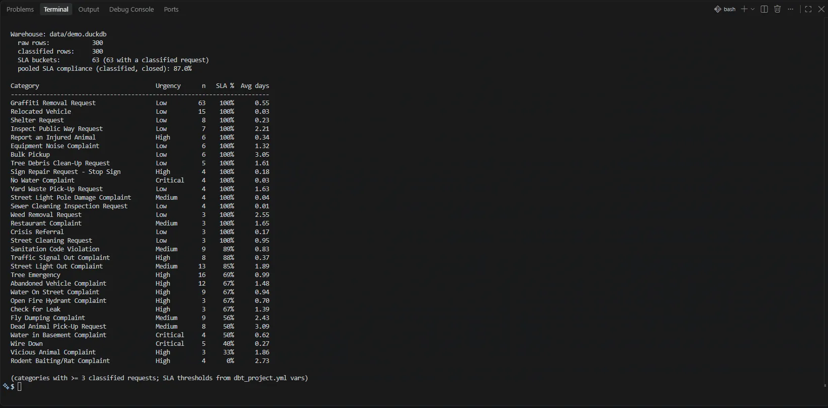
A metric that looked right and wasn’t. The first SLA marts measured compliance over requests that had already closed. The backfill pulled the last seven days of closed requests, and the numbers looked healthy: 87.0% pooled, and the Low tier at 153 of 153. That last figure was the tell. A request opened in the last week and already closed has, by construction, closed inside 168 hours. The slow requests weren’t failing the metric; they were still open, so they weren’t in it.

The fix was to change the denominator, in SQL. The cohort model takes every request created in the fiscal year and gives it a state: met if it closed within its threshold, missed if it closed late or is still open past the deadline, pending if it is open and not yet due, excluded for duplicates, cancellations and four types the city closes at intake. The states partition the created requests, and a test asserts that they do in every bucket. Over FY2026, closed-only measurement says 51.0% and the cohort says 44.8% — closed-only overstates compliance by 6.2 points. The error runs one way: 85 of the 100 in-scope categories look better closed-only, and none look worse. It is largest in the Low tier, 63.2% against 51.1%, where 73,433 requests were still open past their deadline. Both numbers are published side by side.

The headline finding rested on the model’s label. The sharpest result in the first marts was rodent baiting: classified High, held to 24 hours, closed inside that window 0 of 4 times. Then I labelled a blind random sample of 50 requests myself and put both rodent requests at Medium. The SQL had no bug; its input was a judgement, and a metric computed over a model’s labels inherits the labels’ error. On the full fiscal year the gap holds at scale — 18.1% within 24 hours across 41,502 requests — but it still depends on the tier, which a human labelled one level lower.

A green build over an empty mart. Every SLA number on the streaming path derives from updated_datetime, and the intermediate model drops rows where it doesn’t parse. With that field renamed, fct_sla_compliance built with zero rows and all 24 dbt nodes passed — not-null and uniqueness tests are trivially true on an empty table. A tripwire test now fails the build when more than 1% of closed rows lack a parseable close time, and a pytest proves it fails on exactly that test and skips the 13 nodes downstream.

How it’s verified

Check	Result
Clean clone in CI: install, pytest, dbt build on both fixtures	Passes on every push, about a minute
pytest	61 tests, grouped by failure mode: upstream errors, schema drift, DLQ routing, idempotency, portal paging and counts, metric correctness
dbt data tests	45, including the close-time tripwire, seven portal reconciliations and one warn-level date check
Fiscal-year load	2,124,780 rows; 365 of 365 days verified, portal count before and after = rows landed
Portal reconciliations	Cohort denominators = created counts; running totals = an independent monthly group-by; quarters sum to the year; latest version wins; weekly backlog obeys open = previous + opened − closed
Schema drift at ingest	10 scenarios — renamed, missing and new keys, reformatted timestamps, non-object records, a changed envelope
Full Kafka path	300 published, 300 consumed, 0 to the DLQ, on two consecutive runs
Classifier against blind hand-labels	n = 50: 54% exact, 98% within one tier, Cohen’s κ 0.32, quadratic-weighted κ 0.64

The hand-labels were drawn with a fixed seed, made without seeing the model’s answers, and committed before scoring. Graffiti removal is 14 of the 50 rows and agrees on 13; without it, exact agreement is 39%. The disagreements are almost all one tier apart and lean one way: the model was less urgent than the human 15 times and more urgent 8, most often at the Low/Medium line, where the v1 rubric’s own examples overlap.

Parent links are resolved too. All 91,600 come from duplicates. 2,592 parents were created before the fiscal year and are found by ID: an artifact of the extract window. Another 1,066 parent IDs don’t exist in the public portal even when queried one at a time, and 766 of them carry FY2026 numbers, so the window doesn’t explain them. Both counts are published.

What I’d do differently

Build the evaluation before the marts. The SLA marts shipped in May; the first measure of whether the labels behind them were right came four months later, and it changed the headline.

Define the metric’s denominator before its numerator. Closed-only compliance was easy to compute and easy to believe, and it took a full year of data and a cohort to show how much it flattered the city.

Limits

Category triage. The feed has no description text, so requests in the same category mostly receive the same tier, and the fiscal-year marts use one tier per service type by design.

The streaming sample is small. One week and 300 labels; per-category percentages there rest on small counts and are reported closed-only, labelled as such.

The fiscal year is a snapshot. Compliance is as of the 2026-10-06 extract; 1,365 requests were still pending, and later re-pulls will move open requests to closed.

The SLAs are the project’s. The 4 / 24 / 72 / 168-hour thresholds are defined per tier in dbt_project.yml; they are not the city’s commitments.

Evaluation scope. 50 items, one labeller, labelled from the service name. The sample contains no request the model called Critical, so Critical precision is unmeasured, and labeller self-consistency has not yet been re-checked.

Throughput and warehouses. One consumer classifies sequentially at about 0.8 requests a second, with no load testing. The portal path writes DuckDB only; its models compile for Snowflake but haven’t run there.

Links

The repository is linked at the top of this page. Its README has the no-credentials quickstart and a recording of the demo; docs/A2-FISCAL-YEAR.md holds the fiscal-year results and decisions; ARCHITECTURE.md walks through both paths; eval/RESULTS.md holds the confusion matrix and every disagreement with the model’s reasoning.